Section 15.4 Monoids and Machines
¶In this section, we will see how every finite-state machine has a monoid associated with it and how we can represent any monoid with a finite-state machine.
Subsection 15.4.1 The Monoid of a Finite-State Machine
¶For any finite-state machine, the elements of its associated monoid correspond to certain input sequences. Because only a finite number of combinations of states and inputs is possible for a finite-state machine there is only a finite number of input sequences that summarize the machine. This idea is illustrated best with a few examples.
Consider the parity checker. The following table summarizes the effect on the parity checker of strings in \(B^1\) and \(B^2\text{.}\) The row labeled “Even” contains the final state and final output as a result of each input string in \(B^1\) and \(B^2\) when the machine starts in the even state. Similarly, the row labeled “Odd” contains the same information for input sequences when the machine starts in the odd state.
Note how, as indicated in the last row, the strings in \(B^2\) have the same effect as certain strings in \(B^1\text{.}\) For this reason, we can summarize the machine in terms of how it is affected by strings of length 1. The actual monoid that we will now describe consists of a set of functions, and the operation on the functions will be based on the concatenation operation.
Let \(T_0\) be the final effect (state and output) on the parity checker of the input 0. Similarly, \(T_1\) is defined as the final effect on the parity checker of the input 1. More precisely,
while
In general, we define the operation on a set of such functions as follows: if \(s\text{,}\) \(t\) are input sequences and \(T_s\) and \(T_t\text{,}\) are functions as above, then \(T_s*T_t=T_{st}\text{,}\) that is, the result of the function that summarizes the effect on the machine by the concatenation of \(s\) with \(t\text{.}\) Since, for example, 01 has the same effect on the parity checker as 1, \(T_0*T_1=T_{01}=T_1\text{.}\) We don't stop our calculation at \(T_{01}\) because we want to use the shortest string of inputs to describe the final result. A complete table for the monoid of the parity checker is \(\begin{array}{c|c} * & \begin{array}{cc} T_0 & T_1 \\ \end{array} \\ \hline \begin{array}{c} T_0 \\ T_1 \\ \end{array} & \begin{array}{cc} T_0 & T_1 \\ T_1 & T_0 \\ \end{array} \\ \end{array}\)
What is the identity of this monoid? The monoid of the parity checker is isomorphic to the monoid \(\left[\mathbb{Z}_2; +_2\right]\text{.}\)
This operation may remind you of the composition operation on functions, but there are two principal differences. The domain of \(T_s\) is not the codomain of \(T_t\) and the functions are read from left to right unlike in composition, where they are normally read from right to left.
You may have noticed that the output of the parity checker echoes the state of the machine and that we could have looked only at the effect on the machine as the final state. The following example has the same property, hence we will only consider the final state.
Example 15.4.1.
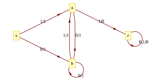
The transition diagram for the machine that recognizes strings in \(B*\) that have no consecutive 1's appears in Figure 15.4.2. Note how it is similar to the graph in Figure 13.1.4. Only a “reject state” has been added, for the case when an input of 1 occurs while in State \(a\text{.}\) We construct a similar table to the one in the previous example to study the effect of certain strings on this machine. This time, we must include strings of length 3 before we recognize that no “new effects” can be found.
\(\begin{array}{ccccccccccccccc} \textrm{ Inputs} & 0 & 1 & 00 & 01 & 10 & 11 & 000 & 001 & 010 & 011 & 100 & 101 & 110 & 111 \\ s & b & a & b & a & b & r & b & a & b & r & b & a & r & r \\ a & b & r & b & a & r & r & b & a & b & r & r & r & r & r \\ b & b & a & b & a & b & r & b & a & b & r & b & a & r & r \\ r & r & r & r & r & r & r & r & r & r & r & r & r & r & r \\ \textrm{ Same} \textrm{ as} & & & 0 & & & & 0 & 01 & 0 & 11 & 10 & 1 & 11 & 11 \\ \end{array}\)
The following table summarizes how combinations of the strings \(0,1,01,10, \textrm{ and } 11\) affect this machine.
All the results in this table can be obtained using the previous table. For example,
Note that none of the elements that we have listed in this table serves as the identity for our operation. This problem can always be remedied by including the function that corresponds to the input of the null string, \(T_{\lambda }\text{.}\) Since the null string is the identity for concatenation of strings, \(T_sT_{\lambda }=T_{\lambda }T_s=T_s\) for all input strings \(s\text{.}\)
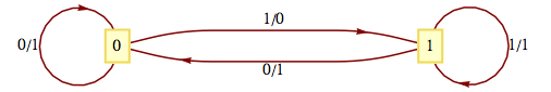
Example 15.4.3. The Unit-time Delay Machine.
A finite-state machine called the unit-time delay machine does not echo its current state, but prints its previous state. For this reason, when we find the monoid of the unit-time delay machine, we must consider both state and output. The transition diagram of this machine appears in Figure 15.4.4.
\(\begin{array}{c|c} \textrm{ Input} & \begin{array}{cccccccccc} & \begin{array}{cc} 0 & 1 \\ \end{array} & 00\textrm{ } & 01\textrm{ } & \textrm{ }10\textrm{ } & 11 & 100\textrm{ or}000\textrm{ } & 101\textrm{ or}001 & 110\textrm{ or}101 & 111\textrm{ or}011 \\ \end{array} \\ \hline \begin{array}{c} 0 \\ 1 \\ \textrm{ Same} \textrm{ as} \\ \end{array} & \begin{array}{cccccccccc} (0,0) & (1,0) & (0,0) & (1,0) & (0,1) & (1,1) & (0,0) & (1,0) & (0,1) & (1,1) \\ (0,1) & (1,1) & (0,0) & (1,0) & (0,1) & (1,1) & (0,0) & (1,0) & (0,1) & (1,1) \\ & & & & & & 00 & 01 & 10 & 11 \\ \end{array} \\ \end{array}\)
Again, since no new outcomes were obtained from strings of length 3, only strings of length 2 or less contribute to the monoid of the machine. The table for the strings of positive length shows that we must add \(T_{\lambda }\) to obtain a monoid.
Subsection 15.4.2 The Machine of a Monoid
¶Any finite monoid \([M;*]\) can be represented in the form of a finite-state machine with input and state sets equal to \(M\text{.}\) The output of the machine will be ignored here, since it would echo the current state of the machine. Machines of this type are called state machines. It can be shown that whatever can be done with a finite-state machine can be done with a state machine; however, there is a trade-off. Usually, state machines that perform a specific function are more complex than general finite-state machines.
Definition 15.4.5. Machine of a Monoid.
If \([M;*]\) is a finite monoid, then the machine of \(M\text{,}\) denoted \(m(M)\text{,}\) is the state machine with state set \(M\text{,}\) input set \(M\text{,}\) and next-state function \(t : M\times M \to M\) defined by \(t(s, x) = s * x\text{.}\)
Example 15.4.6.
We will construct the machine of the monoid \(\left[\mathbb{Z}_2;+_2\right]\text{.}\) As mentioned above, the state set and the input set are both \(\mathbb{Z}_2\text{.}\) The next state function is defined by \(t(s, x) = s +_2 x\text{.}\) The transition diagram for \(m\left(\mathbb{Z}_2\right)\) appears in Figure 15.4.7. Note how it is identical to the transition diagram of the parity checker, which has an associated monoid that was isomorphic to \(\left[\mathbb{Z}_2;+_2\right].\)
![The machine of \([\mathbb{Z}_2;+_2]\)](images/fig-machine-of-z2.png)
Example 15.4.8.
The transition diagram of the monoids \(\left[\mathbb{Z}_2;\times _2\right]\) and \(\left[\mathbb{Z}_3;\times _3\right]\) appear in Figure 15.4.9.
![The machines of \([\mathbb{Z}_2; \times_2]\) and \([\mathbb{Z}_3;\times_3]\)](images/fig-machine-of-zx2-zx3.png)
Example 15.4.10.
Let \(U\) be the monoid that we obtained from the unit-time delay machine (Example 15.4.3). We have seen that the machine of the monoid of the parity checker is essentially the parity checker. Will we obtain a unit-time delay machine when we construct the machine of \(U\text{?}\) We can't expect to get exactly the same machine because the unit-time delay machine is not a state machine and the machine of a monoid is a state machine. However, we will see that our new machine is capable of telling us what input was received in the previous time period. The operation table for the monoid serves as a table to define the transition function for the machine. The row headings are the state values, while the column headings are the inputs. If we were to draw a transition diagram with all possible inputs, the diagram would be too difficult to read. Since \(U\) is generated by the two elements, \(T_0\) and \(T_1\text{,}\) we will include only those inputs. Suppose that we wanted to read the transition function for the input \(T_{01}\text{.}\) Since \(T_{01}=T_0T_1\text{,}\) in any state \(s, t\left(s, T_{01}\right) = t\left(t\left(s, T_0\right), T_1\right).\) The transition diagram appears in Figure 15.4.11.
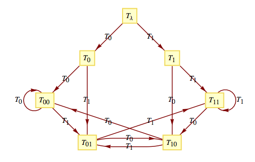
If we start reading a string of 0's and 1's while in state \(T_{\lambda }\) and are in state \(T_{ab}\) at any one time, the input from the previous time period (not the input that sent us into \(T_{ab}\text{,}\) the one before that) is \(a\text{.}\) In states \(T_{\lambda }, T_0\) and \(T_1\text{,}\) no previous input exists.
Exercises 15.4.3 Exercises
¶1.
For each of the transition diagrams in Figure 12, write out tables for their associated monoids. Identify the identity in terms of a string of positive length, if possible.
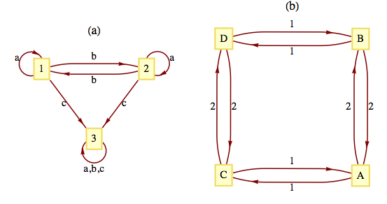
Where the output echoes the current state, the output can be ignored.
-
\(\begin{array}{c|cccccc} \textrm{ Input String} & a & b & c & aa & ab & ac \\ \hline 1 & (a,1) & (a,2) & (c,3) & (a,1) & (a,2) & (c,3) \\ 2 & (a,2) & (a,1) & (c,3) & (a,2) & (a,1) & (c,3) \\ 3 & (c,3) & (c,3) & (c,3) & (c,3) & (c,3) & (c,3) \\ \end{array}\) \(\begin{array}{c|cccccc} \textrm{ Input String} & ba & bb & bc & ca & cb & cc \\ \hline 1 & (a,2) & (a,1) & (c,3) & (c,3) & (c,3) & (c,3) \\ 2 & (a,1) & (a,2) & (c,3) & (c,3) & (c,3) & (c,3) \\ 3 & (c,3) & (c,3) & (c,3) & (c,3) & (c,3) & (c,3) \\ \end{array}\)
We can see that \(T_aT_a= T_{\textrm{ \textit{aa}}}=T_a\text{,}\) \(T_aT_b= T_{\textrm{ \textit{ab}}}= T_b\text{,}\) etc. Therefore, we have the following monoid:
\begin{equation*} \begin{array}{c|c} & \begin{array}{ccc} T_{a} & T_b & T_b \\ \end{array} \\ \hline \begin{array}{c} T_a \\ T_b \\ T_c \\ \end{array} & \begin{array}{ccc} T_a & T_b & T_c \\ T_b & T_a & T_c \\ T_c & T_c & T_c \\ \end{array} \\ \end{array} \end{equation*}Notice that \(T_a\) is the identity of this monoid.
-
\(\begin{array}{c|cccccc} \textrm{Input String} & 1 & 2 & 11 & 12 & 21 & 22 \\ \hline A & C & B & A & D & D & A \\ B & D & A & B & C & C & B \\ C & A & D & C & B & B & C \\ D & B & C & D & A & A & D \\ \end{array}\)
\(\begin{array}{c|cccccccc} \textrm{Input String} &111 & 112 & 121 & 122 & 211 & 212 & 221 & 222 \\ \hline A & C & B & B & C & B & C & C & B \\ B & D & A & A & D & A & D & D & A \\ C & B & C & C & B & C & B & B & C \\ D & B & C & C & B & C & B & B & C \\ \end{array}\)
We have the following monoid:
\begin{equation*} \begin{array}{c|c} & \begin{array}{cccc} T_1 & T_2 & T_{11} & T_{12} \\ \end{array} \\ \hline \begin{array}{c} T_1 \\ T_2 \\ T_{11} \\ T_{12} \\ \end{array} & \begin{array}{cccc} T_{11} & T_{12} & T_1 & T_2 \\ T_b & T_{11} & T_2 & T_1 \\ T_1 & T_2 & T_{11} & T_{12} \\ T_2 & T_1 & T_{12} & T_{11} \\ \end{array} \\ \end{array} \end{equation*}Notice that \(T_{11}\) is the identity of this monoid.
2.
What common monoids are isomorphic to the monoids obtained in the previous exercise?
3.
Can two finite-state machines with nonisomorphic transition diagrams have isomorphic monoids?
Yes, just consider the unit time delay machine of Figure 15.4.4. Its monoid is described by the table at the end of Section 14.4 where the \(T_{\lambda }\) row and \(T_{\lambda }\) column are omitted. Next consider the machine in Figure 15.4.11. The monoid of this machine is:
Hence both of these machines have the same monoid, however, their transition diagrams are nonisomorphic since the first has two vertices and the second has seven.
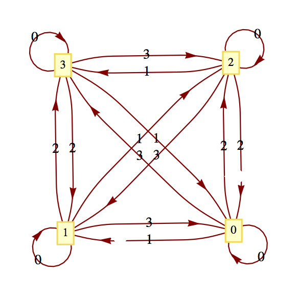
3.
Draw the transition diagrams for the machines of the following monoids:
\(\left[\mathbb{Z}_4;+_4\right]\)
The direct product of \(\left[\mathbb{Z}_2;\times _2\right]\) with itself.
4.
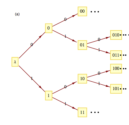
Even though a monoid may be infinite, we can visualize it as an infinite-state machine provided that it is generated by a finite number of elements. For example, the monoid \(B^*\) is generated by 0 and 1. A section of its transition diagram can be obtained by allowing input only from the generating set. The monoid of integers under addition is generated by the set \(\{-1, 1\}\text{.}\) The transition diagram for this monoid can be visualized by drawing a small portion of it, as in Figure 15. The same is true for the additive monoid of integers, as seen in Figure 16.
![An infinite machine \([\mathbb{Z};+]\)](images/fig-exercise-15-4-2b.png)
Draw a transition diagram for \(\{a, b, c\}\)
Draw a transition diagram for \([\mathbb{Z}\times \mathbb{Z};\textrm{componentwise addition}]\text{.}\)
Draw a transition diagram for \([\mathbb{Z};+]\) with generating set \(\{5,-2\}\text{.}\)